When an area on an imager is “uniformly”
illuminated there will be some spatial and temporal variation in pixel value
due to quantum  effects. Figure 1 is a representation of this variation. The pixel to pixel variation in the number of
photons collected at each pixel for “uniform” illumination varies with a
Poisson distribution. A Poisson distribution looks like a normal distribution except
the values are discrete and they are skewed left up to an average value of about ten counts. At average values larger than ten
counts a Poisson distribution closely matches a normal distribution except the values are discrete.
The standard deviation for a Poisson distribution is the square root of the average number
of photons collected. The pixel to pixel standard deviation equals
the square root of the average number of photons collected over a large number
of pixels.
effects. Figure 1 is a representation of this variation. The pixel to pixel variation in the number of
photons collected at each pixel for “uniform” illumination varies with a
Poisson distribution. A Poisson distribution looks like a normal distribution except
the values are discrete and they are skewed left up to an average value of about ten counts. At average values larger than ten
counts a Poisson distribution closely matches a normal distribution except the values are discrete.
The standard deviation for a Poisson distribution is the square root of the average number
of photons collected. The pixel to pixel standard deviation equals
the square root of the average number of photons collected over a large number
of pixels.
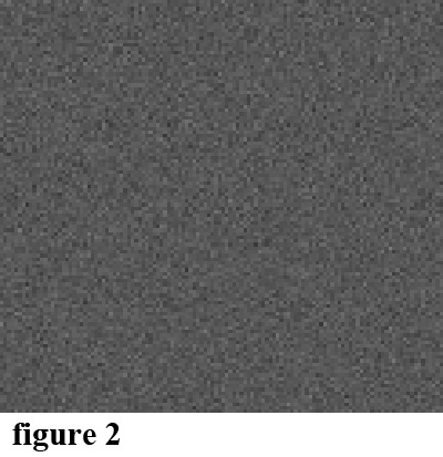
Each pixel in an imager acts like a bin that collects photons and converts them to electrons, for the moment it will be assumed that all the photons get converted to electrons. The smaller the area of the bins (pixel size), the shorter the collection time (exposure time), or the lower the image illumination (scene illumination or f/number) the fewer photons each bin collects. An example of an image patch with Poisson noise is shown in figure 2.
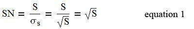
By definition the signal to noise (SN) equals the signal
divided by the signal standard deviation. The SN is determined for an image by measuring the average value of a uniform patch and dividing by the standard deviation for the patch. The standard deviation of a Poisson limited signal is the square root of the signal. Equation (1) shows that for a Poisson limited signal the SN equals the square root of the signal. 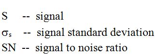
 A full image noise simulation includes additional noise
sources including read noise, dark signal non-uniformity (DSNU), dark current, and
pixel response non-uniformity (PRNU), but for some purposes it is useful to
look at one noise source at a time. Poisson noise is interesting because even if
all of the process dependent noise sources are zero Poisson noise will still be
present. The monochrome simulations below only
include Poisson noise.
A full image noise simulation includes additional noise
sources including read noise, dark signal non-uniformity (DSNU), dark current, and
pixel response non-uniformity (PRNU), but for some purposes it is useful to
look at one noise source at a time. Poisson noise is interesting because even if
all of the process dependent noise sources are zero Poisson noise will still be
present. The monochrome simulations below only
include Poisson noise.
 A photon is characterized by a certain amount of
energy. In radiometric units this
corresponds to a joule or equivalently a watt-second. In photometric units a watt-second
corresponds to a lumen-second with a wavelength dependent scaler. The
number of lumen-seconds per area falling on an imager in a camera depends on
the ISO exposure setting. The camera
will adjust the exposure time and f/number to expose the imager to a certain
number of lumen-seconds per area which corresponds to a certain number of
photons per area depending on the spectral distribution of the light source.
A photon is characterized by a certain amount of
energy. In radiometric units this
corresponds to a joule or equivalently a watt-second. In photometric units a watt-second
corresponds to a lumen-second with a wavelength dependent scaler. The
number of lumen-seconds per area falling on an imager in a camera depends on
the ISO exposure setting. The camera
will adjust the exposure time and f/number to expose the imager to a certain
number of lumen-seconds per area which corresponds to a certain number of
photons per area depending on the spectral distribution of the light source.
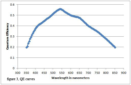
Imagers are more efficient at converting some wavelengths (colors) of light to electrons than others. The quantum efficiency (QE) curve in figure 3 shows the QE at each wavelength. Quantum efficiency is the number of electrons generated at a pixel divided by the number of photons falling on the pixel.
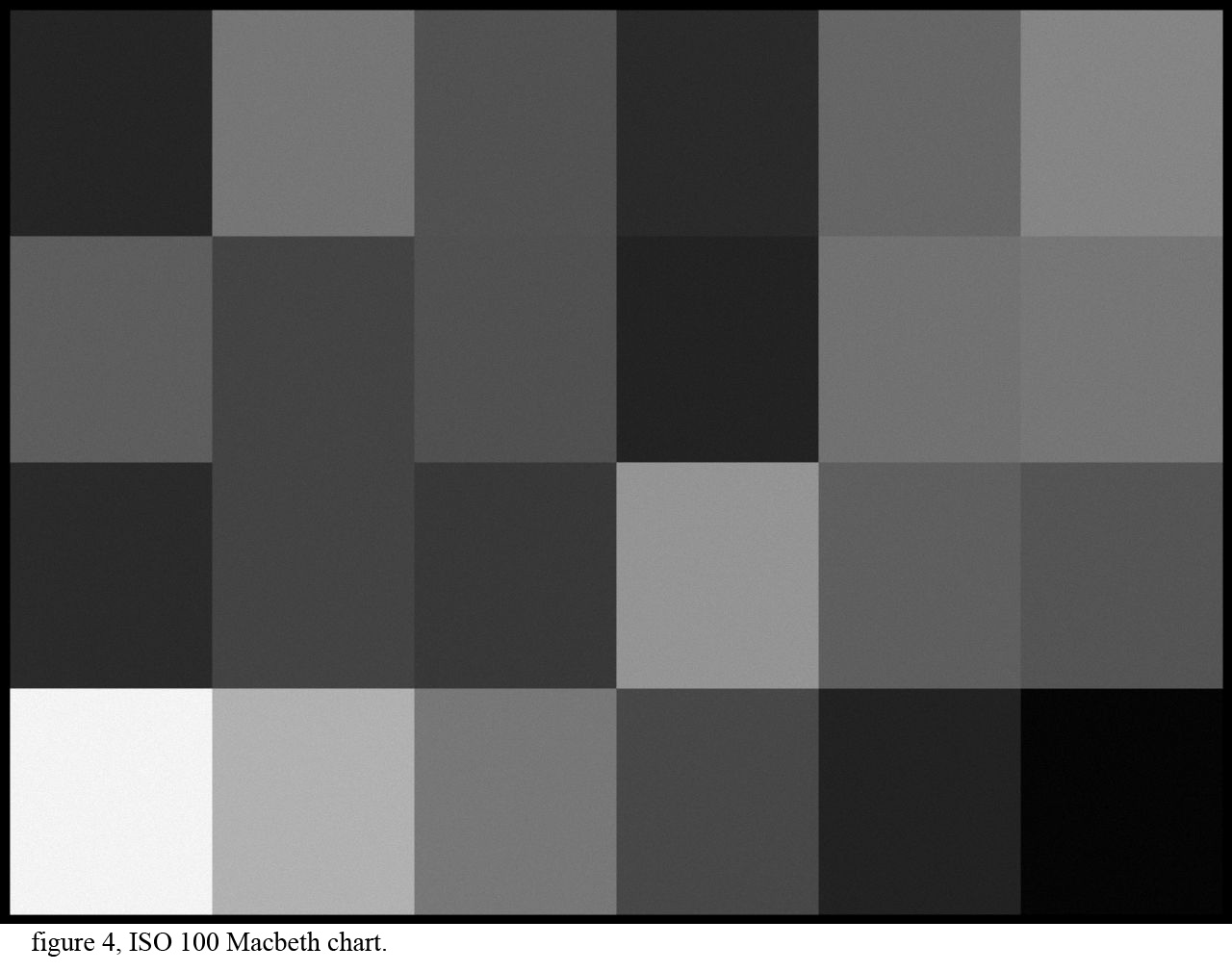
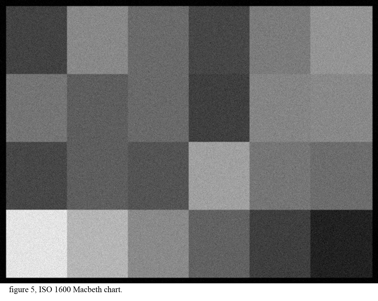
The images below are simulated monochrome images of a 24 patch Macbeth target with Poisson noise. The pixel size is 1.5 micron square. The images are 640 by 480 pixels. Notice the ISO 100 image has much lower noise than the ISO 1600 image because each pixel collects more photons at ISO 100.